
Quantum Computing Modalities
A Qubit Primer Re-Revisited in December 2024

In December 2021, in an early iteration of this Blog, I described the various qubit modalities in use by some of the Quantum Computing (QC) hardware players and then updated that analysis again in October of 2022. You can view that post here (it has been, by far, my most popular post to-date on LinkedIn). A lot has happened since that post, so I thought it would be constructive to revisit the topic again.
When that first post was published, it described 10 leading quantum hardware companies focusing on four core qubit types (superconducting, trapped ions, photonics and quantum dots). In the 2022 update there were 26 quantum hardware companies covered and the addition of neutral atoms and today there are many dozens of quantum hardware companies, and a few additional modalities (notably NV Diamonds and Topological) and significant advances made across the spectrum.
Qubit Dynamics
While many articles describing and comparing QCs focus on the number of qubits, this core number belies the complexity in comparing actual QC performance due to additional limitations described below. Qubit count is the equivalent of only using horsepower to describe a car. While horsepower is an important metric, most car buyers are equally if not more focused on comfort, handling, fuel economy, styling, etc. Some effort has been made to “consolidate” these variables for QC into a single performance metric (such as Quantum Volume, CLOPS (circuit layer operations per second), Q-score or other benchmarks), although no single measurement has yet been adopted by the broad QC community. For the casual reader, I’d caution you to not focus too much on the number of qubits a given QC has. While “more is better” is generally a useful mantra, as you’ll see below, it is not that simple.
As you may know or recall, placing qubits in a superposition (both “0” and “1” at the same time) and entangling multiple qubits where one is dependent on the status of the other (entanglement) are two fundamental quantum properties which help empower Quantum Computers and allow them to perform certain calculations that can’t easily be executed on traditional computers. Before we review the various types of qubits (i.e., quantum hardware platforms), it may be helpful to summarize some of the limitations faced when placing qubits in superposition and/or entangling multiple qubits, and discuss the key metrics used to measure these properties.
Two-qubit Gate Error Rate: Entanglement is a core property of QCs and the two-qubit gate error rate is the second-most-often reported metric (after qubit count). An error rate of 1% is the equivalent of 99% gate fidelity. You may have come across the concept of a ‘CNOT gate’ or controlled-not gate, which uses two qubits and when the first (control qubit) is in a desired state, it flips the second (target qubit). While this sounds basic and simplistic, it is this correlating of the qubits that enables the exponential speedup of QCs. Said another way, it is a method for enabling QCs to analyze multiple pathways simultaneously and so is truly a fundamental property being leveraged by QCs. Many in the industry suggest that 2Q fidelities exceeding 99.99% will be required to achieve quantum advantage and some modalities are approaching that (for example, IonQ and Quantinuum have each exceeded 99.9%).
Single qubit/Rotation Error Rate: Single qubit gates, also often referred to as “rotations” adjust the qubits around various axes (i.e., x-axis, y-axis, and z-axis). In classical computing, you may be familiar with a NOT gate, which essentially returns the opposite of whatever is read by the machine. So, a NOT applied to a 0, “flips” it to a 1. Similarly, in quantum computing, we have the X-Gate, which rotates the qubit 180-degrees (around the X-axis) and so also takes a 0 and “flips” it to a 1. Given the exquisite control required to manipulate qubits, it is possible that the pulse instructing the qubit to “flip” may only apply 179-degress of rotation instead of the required 180 and therefore lead to some error, especially if such imprecision impacts many qubits within an algorithm.
Decoherence Time (T1 and T2): T1 (qubit lifetime) and T2 (qubit coherence time) are effectively two ways to view equivalent information, namely “how long do the qubits remain in a state useful for computation?” Specifically, T1 measures a qubit lifetime, or for how long we can distinguish a 1 from a 0 (time before a bit-flip error), while T2 is focused on phase coherence (time before a phase-flip error), a more subtle but also crucial aspect of qubit performance. Many early QC modalities such as superconducting have modest T2 lifetimes, capping out at 100 microseconds (or millionths of a second) whereas some recent entrants such as neutral atoms, have achieved T2 as long as 10 seconds and certain trapped ions have extended that to 60 seconds. These many orders of magnitude difference in T2 among qubit modalities are a key differentiator among them.
Gate Speed: Is a metric that measures how quickly a QC can perform a given quantum gate. This is especially important relative to the decoherence time noted above, in that the QC must implement its gates BEFORE the system breaks down or decoheres. Gate speed will become increasingly important as a raw metric of time-to-solution where microseconds add up. Interestingly, the modalities with relatively short T2 times (i.e., superconducting, and photonic) generally have the fastest gate speeds (20 MHz – 100 MHz, or 20 million to 100 million operations per second). And while trapped ion gate speeds are much slower, this metric continues to improve (and now can operate at up 1 KHz or 1,000 operations per second).
Connectivity: Sometimes referred to as topology, is a general layout of the qubits in a grid and is concerned with how many neighboring qubits a given qubit can interact with. In many standard layouts, the qubits are lined up in rows and columns with each qubit able to connect to its four “nearest neighbors”. Other systems can have “all-to-all” qubit connectivity, meaning every qubit is connected to every other one. If two qubits can’t directly interact with each other, “swaps” can be inserted, to move the information around and enable virtual connections, however this leads to added overhead, which translates into increased error rates.
SPAM (State Preparation and Measurement) Error Rate: At the start of any quantum algorithm, the user must first set the initial state, and then in the end, that user must measure the result. SPAM error measures the likelihood of a system doing this correctly. A 1% SPAM error on a five-qubit system provides a very high likelihood that the results will be read correctly (99%5=95%) but as the system scales, this becomes more problematic.
Qubit Modalities
When the bits created for classical computing were first created, there were several different transistor designs developed. Similarly, today there are many ways to create a qubit and there are crucial performance trade-offs among them. The following is a brief overview of some of the more common types:
Superconducting Qubits:
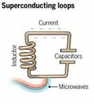
Some leading Quantum Computing firms including Google and IBM are using superconducting transmons as qubits, the core of which is a Josephson Junction which consists of a pair of superconducting metal strips separated by a tiny gap of just one nanometer (which is less than the width of a DNA molecule). The superconducting state, achieved at near absolute-zero temperatures, allows a resistance-free oscillation back and forth around a circuit loop. A microwave resonator then excites the current into a superposition state and the quantum effects are a result of how the electrons then cross this gap. Superconducting qubits have been used for many years so there is abundant experimental knowledge, and they appear to be quite scalable. However, the requirement to operate near absolute zero temperature adds a layer of complexity and makes some of the measurement instrumentation difficult to engineer due to the low temperature environment.
Trapped Ions:
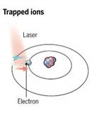
Another common qubit construct utilizes the differential in charge that certain elemental ions exhibit. Ions are normal atoms that have gained or lost electrons, thus acquiring an electrical charge. Such charged atoms can be held in place via electric fields and the energy states of the outer electrons can be manipulated using lasers to excite or cool the target electron. These target electrons move or “leap” (the origin of the term “quantum leap”) between outer orbits, as they absorb or emit single photons. These photons are measured using photo-multiplier tubes (PMT’s) or charge-coupled device (CCD) cameras. Trapped Ions are highly accurate and stable although are slow to react and need the coordinated control of many lasers.
Photonic Qubits:
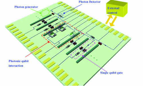
Photons do not have mass or charge and therefore do not interact with each other, making them ideal candidates of quantum information processing. However, this same feature makes two-gate implementation particularly challenging. Photons are manipulated using phase shifters and beam splitters and are sent through a maze of optical channels on a specially designed chip where they are measured by their horizontal or vertical polarity.
Neutral Atoms:

Sometimes referred to as “cold atoms” are built from an array of individual atoms that are trapped in a room-temperature vacuum and chilled to ultra-low temperatures by using lasers as optical “tweezers” to restrict the movement of the individual atoms and thereby chill them. These neutral atoms can be put into a highly excited state by firing laser pulses at them which expands the radius of the outer electron (a Rydberg state), which can be used to entangle them with each other. In addition to large connectivity, neutral atoms can implement multi-qubit gates involving more than 2 qubits, which is instrumental in several quantum algorithms (i.e., Grover search) and highly efficient for Toffoli (CCNOT) gates.
Silicon Spin/Quantum Dots:
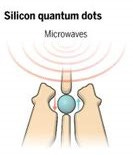
A quantum dot is a nanoparticle created from any semiconductor material such as cadmium sulfide, germanium, or similar elements, but most often from silicon (due to the large amount of knowledge derived from decades of silicon chip manufacturing in the semiconductor industry). Artificial atoms are created by adding an electron to a pure silicon atom which is held in place using electrical fields. The spin of the electron is then controlled and measured via microwaves.
Diamond Vacancies:
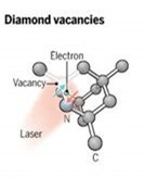
Also known as nitrogen-vacancy centers (NV diamonds) involve tiny imperfections in a diamond’s crystal lattice whereby some of the carbon atoms are replaced by nitrogen. This unique configuration allows an environment where individual electrons can be trapped and manipulated, all at room temperature and with very long coherence times.
Topological:

a nanowire of a semiconductor that has strong spin-orbit coupling is placed in contact with an s-wave superconductor, such as aluminum, in the presence of an external magnetic field B. The nanowire device experiences a topological phase with decaying Majorana bound states at both ends (Majorana Zero Modes or MZMs). To perform computations, the positions of the MZMs are manipulated in a process called “braiding” which is analogous to weaving strands in a braid. Because this form of qubit involves physical encoding (i.e., braiding) it is more resilient to outside noise (i.e., decoherence).
The following table highlights some of the features of more common qubit modalities, as of Dec. 2024:

There are a few other modalities including Nuclear Magnetic Resonance, and Quantum Annealing (used by D-Wave, one of the first firms to offer commercial “Quantum” computers, but annealing is not a true gate-capable construct) and analog versions of neutral atom computing (also not gate-capable). It is likely that more methodologies will be developed.
The following table summarizes some of the benefits and challenges along with select current proponents of key qubit technologies currently in use:

The table above is not intended to be all-inclusive (apologies in advance for any omissions) and some companies are working on multiple modalities (e.g. Intel is working on superconducting as well as silicon spin, and Alice & Bob have a unique approach to superconducting where they add photons to create cat qubits). In fact, there is an excellent compendium of qubit technologies put out by Doug Finke’s Quantum Computing Report which can be accessed here (behind a pay wall, but well worth the fee), and which includes over 150 different quantum hardware computing programs/efforts. There is also a great listing of QPU metrics on the Quantum Insider website which you can see here.
Conclusions
As noted in this post, there have been significant advancements in Quantum Computing hardware over the past year or two and I expect this momentum will continue in 2025. Presently there are QCs with as many as 1,2000 qubits, and the coherence, connect-ability and control on these early machines continues to improve. In 2025 I expect to see more headlines focused on qubit quality and error correction as opposed to focusing on numbers of qubits. Adding sophisticated control and algorithm compilation further extends the capability of these early machines. Whether and when we can achieve universally recognized quantum advantage (i.e., these QCs performing operations that existing supercomputers cannot do) during this NISQ (noisy intermediate stage quantum) era remains to be seen, but this author believes there will be some modest commercial utility squeezed out of these machines in 2025 and is excited to continue tracking (and reporting on) the progress.
Disclosure: The author has modest positions in some stocks discussed in this review but does not have any direct business relationship with any company mentioned in this post. The views expressed herein are solely the views of the author and are not necessarily the views of Corporate Fuel Partners or any of its affiliates. Views are not intended to provide, and should not be relied upon for, investment advice.
References:
Qubit images from Science, C. Bickel, December 2016, Science, V. Altounian, September 2018, New Journal of Physics, Lianghui, Yong, Zhengo-Wei, Guang-Can and Xingxiang, June 2010.
Performance Tables and additional modality details from Quantum Computing Report
Qubit Implementation Dashboard and The Quantum Insider Quantum Processors table, both accessed December 2024.
Blank, Steve, Quantum Computing - An Update, October 22, 2024.
Bobier, Langione, Tao and Gourevitch, “What Happens When ‘If’ Turns to ‘When’ in Quantum Computing?”, BCG, July 2021.
“Comparing Quantum Computers: Metrics and Monroney,” IonQ, February 18, 2022.
Henriet, L., Beguin, L., et. al., “Quantum Computing with Neutral Atoms,” arXiv:2006.1232v2 [quant-ph], September 18, 2020.
Lichfield, Gideon, “Inside the race to build the best quantum computer on Earth”, MIT Technology Review, February 26, 2020.
Ray, Amit, “7 Primary Qubit Technologies for Quantum Computing”, December 10, 2018.
Silverio, H., Grijalva, S, et. al., “Pulser: An open-source package for the design of pulse sequences in programmable neutral-atom arrays,” arXiv:2104.15044v3 [quant-ph], January 12, 2022.
